

ABSTRACT
The purpose of the study was to examine the physicochemical characteristics and the level of metalloid pollution in the Bhairab River. This study used the Heavy Metal Contamination Index (HPI) and for an extensive examination. The single factor indexing approach was used to determine the distribution pattern of pollution at sample stations by specific metalloid contaminants. The sample was taken during high tide and low tide in the wet season and dry season. Based on consistent spacing between them and the establishment of economic operations that significantly contribute to pollution along the riverbank, five sampling stations were chosen. Thirty samples in all, including duplicates, were gathered. Prior to being sent to the laboratory to determine their content, the samples were digested in accordance with USEPA 3005 and APHA (1998) standard procedures. The amount of heavy metals in water samples analyzed in the research region grows in the order of Fe > Cu > Pb > Ni > Cr > Mn > Zn > As > Cd during dry season and Fe > Zn > Cu > Mn > Cr > Pb > Cd > As > Ni during wet season. The river water quality indicated that it is suitable for industrial cooling, fish culture, and irrigation. The strong significant positive correlation (r=.642) between Cu and Cd suggests that their sources may be similar. The water deemed unfit for human consumption since the average HPI, which was determined for both research seasons, was higher than 100. The abundance of distinct metalloid characteristics at different sampling locations was also revealed by the single factor pollution index. It was anticipated that the residential waste and irrigation sectors, along with the print and electronics industries, would produce the majority of the effluents, with geogenic sources contributing very little.
CHAPTER ONE – INTRODUCTION
Heavy metals have atomic weight and density minimum five times greater than that of water (Tchounwou, 2012). Because of their numerous industrial, domestic, agricultural, medical, and technical opportunities to practice, they are widely distributed in the environment, prompting worries about their possible effects on human and environment (hydrosphere, lithosphere, biosphere, and atmosphere). Arsenic (As), cadmium (Cd), chromium (Cr), copper (Cu), nickel (Ni), lead (Pb), and mercury (Hg) are the most frequently detected metal pollutants. Specific pollution occurs when pollutants rely on a detectable source. On the other hand, contaminants coming from distant (and frequently ill defined) origins create nonspecific pollution. Pollutants coming from specific manufacturing unit, such as mining, metal based manufacturing operations etc. are particularly problematic for the environment.
Runoff from industries, municipalities and urban areas contribute in the transportation and accumulation of heavy metals in the ecosystem (Musilova, 2016). Because of their longevity, eco toxicity, bioaccumulation, and other factors, these elements are considered to be a major origin of pollution of the hydroshpere (Zhang, 2014; Bryan, 1992; Redwan, 2017; Jordanova, 2018). These metals from insufficiently managed effluent from industries reach aquatic habitats (e.g., lakes, rivers, reservoirs, and wetlands). Pollution caused by this type of metallic elements is creating chaos on rivers all around the globe (Akcay, 2003; Olivares-Rieumont, 2005) particularly in developing countries (Wang, 2011; Li, 2013). Sediment being an intrinsic part of ecosystems governed by rivers, acts as both a source and a supplier of metals having high atomic weight (Pejman, 2015; Huang, 2019). These metals immediately settle in the sediments as soon as they get into the rivers (Shyleshchandran, 2018; Liu, 2018). Thus to assess the pollution level, the studies on river water quality situated near an industry discharging heavy metal containing effluent have achieved a great interest at present time.
The transition from an agricultural and handicraft economy to one dominated by industry and equipment production is known as industrialization. Initially, industrialization efforts in emerging countries were sparse and reluctant. In 1945, this began to alter. In the post war years, developing countries returned to the commercial race after a 50-year hiatus (Balance et al., 1982). Production has been a central task in many emerging countries since WWII, and the formation of industrial production and commerce has drastically altered. The colonial and post – colonial division of labor has been thrown into question. Production has been transferred to relatively under developed countries, which transfer their manufacturing goods to the first world countries. Today’s technology has created significant changes in the world economic growth layout with persistent advances in labor quality and increased welfare (Maddison, 2001; Maddison, 2007). These advancements in technology revolutionized civilization by introducing new approaches to working and dwelling.
The Industrial Revolution had a long-term effect on people’s lifestyles. As the technological advancement paces up, battery industries have been witnessing unavoidable demand as battery is an integral part of any machine. This results in the rise of heavy metal (mainly Pb, Cd, Hg and Ni) pollution through untreated or partially treated effluent discharge, unregulated waste management and natural occurrence like floods, acid rain.
Water is amongst the most significant elements on the planet. The significance of water supplies, notably surface waterways (rivers), in providing the water demands of individuals, livestock, and businesses highlights the critical necessity to safeguard them against pollution. Contamination by heavy metals is now a prime issue in the third world countries, such as Bangladesh. Bangladesh’s unplanned development and commercialization has an adverse consequence on the quality of the aquatic resources.
Impurities in waterways
The impurities come from three main components: i) wastewater dumped into the surface water resources, (ii) untreated wastewater discharged into the river, and (iii) surface runoff from farmlands where synthetic nutrients, chemicals, pesticides, and soil amendments are utilized (Dwivedi, 2017). Industries produce a large amount of sewage, which eventually ends up in streams or rivers. Manufacturing outflows comprising poisonous and hazardous compounds are the main origin of pollution in surface waters. The formation of pollutants, particularly small scale cottage industries that release unprocessed effluents, originated from technological innovation expressed by the introduction of special industries or the improvement of existing industrial operations. Various studies have identified big and small-scale industry sludge, urban runoff, and septic systems as sources of contamination. The quality of wastewaters emitted from various units varies, as do their guidelines, depending on the country (Ragas and Lenven, 1999). Li and Morioka determined the most polluted spot in a waterway when multiple sources intersect transversely (1999).
Edwards et al. investigated a multifaceted feature of water (1989). Dugan’s research has looked for the chemical and biological pollutants of water, as well as their linkages (1972). Urban civilization utilizes more water, and the composition of wastewaters there is chemically more harmful than the rural settlements (Bandy, 1984). The connection between pollution and health issues is now well-established and reasonably well-known to the general population (Barzilay et al., 1999).
Bhairab river
The Bhairab River flows through the Indian state of West Bengal and south-western Bangladesh. The river is an affluent of the Ganges (Rob, 2012). It traverses Khulna, separating it into two sections. The Bhairab River begins at the Tengamari boundary of Meherpur and flows through Jashore (Geology of the Khulna City, 2010). The waterway is roughly 160 kilometers (100 miles) in length and 91 meters (300 feet) in width. Its usual depth is between 1.2 and 1.5 meters (4 to 5 feet), and its water flow is minor. It is rich in silts (Hossain, 1994). This river is extremely significant to Bangladesh’s antiquity. The historical commerce of Bangla revolves around this river. It was also significant during the Moghal Period, when Protapaditto was the Jashore’s landlord. After that, though, the river progressively loses its attractiveness and assumes a more modern appearance. The majority of this river is located in Jashore. The Bhairab River has two major tributaries: The Ichamati and the Kobadak. A portion of the Khulna-Ichamati is located in India, while another portion is in the Satkhira region of Bangladesh; as such, it serves as the border between Bangladesh and India. On the river’s bank are the cities of Khulna and Jashore (Geology of the Khulna City, 2010). It is believed that the Bhairab is older than its parent river, the Jalangi. A few kilometres north of Karimpur, it emerges from the river at a point (in West Bengal). After a circuitous journey to the south, it turns east. For a short distance, it serves as the border between Meherpur P.S. (Bangladesh) and Karimpur (India). The river then turns south and flows past Meherpur town before entering Meherpur P.S. Finally, it disappears into the Mathabhanga near Kapashdanga to the east. The Rupsa River is produced by the confluence of the Bhairab and Atrai rivers and empties into the Pasur (Chowdhury, 2012). Currently, the river cannot be navigated beyond the Bagherpara Upazila in the Jashore district. During the monsoon, the Ganges nourishes it, but during the dry season it dries up. Its lower stream is passable year-round and is influenced by the tides. Meherpur, Chuadanga, Barobazar, Kotchandpur, Chaugachha, Jashore, Daulatpur, Bagerhat, and Khulna are among the significant cities situated along the Bhairab river (Chowdhury, 2012). Bangladesh has a tropical monsoon climate with distinct seasonal differences. The monsoon season (July to October) is followed by a cold winter (November to February), then a hot, dry summer (March-June). Seventy to eighty percent of yearly precipitation falls during the monsoon season (Banglapedia, 2015).
Surrounding commercial activities and effluent discharge
Several enterprises and match manufacturers in the Rupsa industrial region of Khulna are responsible for the contamination of the Rupsa River. Khalishpur’s Khulna Newsprint Mill, Hardboard Mills, Goalpara Thermal Power Station, and Jute and Iron Industries dump all of their garbage into the Bhairab River. The Khulna Newsprint Mill discharges approximately 4,500 cubic meters per hour of effluent containing suspended, undissolved solids into the Bhairab River.
In 2001, according to a recent report, there were 58 manufacturing subdivisions in this region. There are currently approximately 350 industrial units in the region. On the banks of the Bhairab River are 230 industries, including jute mills, power plants, soya bean mills, shrimp processing units, and cement factories. Shipyard, Koraeshi Steel. Mill, Bangladesh Match Factory, Dada Match Factory, Khulna Textile Mill, News Print Mill, Hard Board Mill, Daulatpur Jute Mill, Platinum Jute Mill, Crescent Jute Mill, Peoples Jute Mill, Star Jute Mill, Senhati Re-rolling Mill, Jute Press, Anser Flour Mill, Ajax Jute Mill, Sonali Jute Mill, Mohsin Jute Mill, Cables Factory, more than twenty-two shrimp processing industries contribute to the degradation of the environmental quality of Khulna. Several sea food enterprises are located in the neighbourhood. Various species of organisms are adversely affected by oil contamination in different ways. The thin layer of oil on water decreases inhibits proper light penetration and dissolved oxygen (Texascenter, 1992).
Surface water pollution by harmful metals
According to UNEP/GPA (2006a), an increasing global challenge introduces mismanagement of electronic waste (e-waste), specially dumping of used computers and cell phones, which contain over 1000 distinct elements, many of which are harmful to humans.
Metals such as copper, iron, chromium, and nickel are required because they act as a crucial part for the living system, whereas cadmium and lead are inessential metals since even trace amounts of them are harmful (Fernandes et al., 2008). The fish must absorb the needed metals from water, food, or sediment in order to maintain a normal metabolic rate (Canli and Atli, 2003). These necessary elements can also cause toxicity when consumed in excessive quantities (Tuzen, 2003). In the past decade, studies on metalloid pollution of hydrosphere has been a major concern for the ecosystems (Fernandes et al., 2008; Ozturk et al., 2008; Pote et al., 2008; Praveena et al., 2008). Pesticides play a substantial influence in the transportation of contaminants in aquatic systems under suitable circumstances, as well as in water-sediment interactions (Rashed, 2011). Our country is amongst the most polluted nations, with 1176 enterprises discharging around 0.4 million m3 of untreated garbage every day into the rivers (Rabbani and Sharif, 2005). The deterioration may have been caused by the reckless release of easily oxidized industrial and municipal organic pollutants directly into the rivers (BCAS, 2004).
Effects of metalloid pollution
Heavy metals are available in a wide range of hazardous effluents. Hydrophytes collect these substances (Villar et al., 1999). In the sediments, these substances also precipitate (Gonzalez et al., 2000). Risgard and Hansen found Hg in hydrophytes and herbivorous fishes (1990). Pacakova et al. investigated metal concentration in several layers of rivers (2000). Some plants have been recommended as bio screens because of their ability to absorb nutrients (Reddy and De Busk, 1987). Mayes et al. discovered that rooted aquatic plants accumulate Cd and Pb (1977). In a nutrient-rich lake, Hg, Cd, Pb, and Tl have been found (Mathis and Kavern, 1975). Many types of malignancies, including gall bladder cancer, have been linked to the buildup of harmful metals such as cadmium, copper, and nickel in recent studies.
Different species react differently to metals based on their inert capability; therefore, some species are more tolerant and resistant to metals than others (Akinyemi et al., 2004). In addition, the tenacious nature of certain metals causes them to stay in the ecosystem for a long period of time, posing risks to humans and other organisms. Considering the above features of harmful metals and the increasing pollution in our environment, it is sufficient to conclude that heavy metals pose a grave hazard (Edward et al., 2013).
The harmful effects of metals on living beings are extensive (WHO, 2009; USEPA, 2000), particularly when taken in excess of the limits established by various regulatory authorities. Elements such as arsenic, mercury, and lead may be harmful even at minor exposure intensity. After being ingested by humans, heavy metals continue to accumulate in key organs such as the brain, liver, bones, and kidneys for years, resulting in detrimental health effects (Norris et al., 1993). Ingestion of food polluted with heavy metals can potentially cause a variety of significant health issues. Heavy metal intakes cause a variety of health issues, including immunological impairment, intrauterine development defect, altered psychosocial behavior, and nutritional deficiency (Nweke and Sanders, 2009).
When heavy metals are not metabolized by the body and accumulate in the soft tissues, they become poisonous. Natural and anthropogenic activities are affecting the environment to an extent that it surpasses the aptitude of the ecosystem (Herawati et al., 2000; He et al., 2005).
Effects of seasonal variation in water quality
The US Environmental Protection Agency (EPA) has compiled a number of water quality criteria that can be used to quantify aquatic environment (EPA, 2001). Different metrics, biological, radiological, and physical are used to assess the hydrology (their allowable quantities for each component are established by the World Health Organization and the Food and Agricultural Organization for various reuse purposes) (Alam et al., 2007; Popa et al., 2012).
A report released in 2019 found that the Bhairab river’s estimated water quality parameters ranged higher during the rainy season due to the large volume of freshwater discharge and the reduced impact of tidal flow. The seasonal pollution load index ranked summer > winter > wet season in ascending order (Khan et al., 2019).
Preservation and outflow are complex effects of the physiographic properties of the reservoir (Smakhtin, 2001; Yunus et al., 2003), whereas recharge is mostly dependent on precipitation. Low streamflow caused by climate change, E1-Nino Southern Oscillation (ENSO) occurrences, and droughts has negative physical, chemical, and biological consequences on quality of water and freshwater biology (Burn, 1994; Herrmann et al., 2000; Caruso, 2001).
Streamflow fluctuations can have a variety of geographical and temporal consequences on stream ecosystems, even in limited regions such as watersheds (Jailani et al., 2004). Nonetheless, the amplitude and duration of these parameters’ extreme values, which are typically vital to biota, may rise with extreme low streamflow. In urban and agro based catchments, nonspecific sources of pollution increased during the wet season due to discharge and overflow. The quantity and quality of water parameters are determined by the effects of seasonal fluctuations in streamflow.
Whilst the changing climate can have a range of consequences on streamflow and aquatic habitat, anthropogenic activities found to have a higher influence. Resurfacing watersheds and the concomitant building of manmade channels increases the real influence of precipitation into river systems (Foster et al., 1999). Many rivers in the relatively under developed countries anthropogenic activities result in harmful discharges that contribute in the deterioration of the aquatic environment (Jonnalagadda et al., 1991; Mathuthu et al., 1993; Jonnalagadda and Nenzou, 1996; Bordalo et al., 2001).
Importance of HPI in the assessment of metalloid pollution in surface water
With the introduction of the heavy metal pollution index (HPI) in recent decades, the assessment of metalloid pollution in ground and surface waters has attracted extensive interest (Reddy 1995; Mohan et al., 1996). Metals examined for the evaluation of the quality of any water resource provide an indication of the contamination in relation to that metal alone. HPI is a tool for estimating the mass impact of specific metals on the general quality of water and is necessary for determining the total contribution of all metals to contamination. The HPI takes a close strategy to Horton (1965) and the NSFWQI. In contrast to conventional WQI, in which sub-indices are derived utilizing just standard values, the HPI employs both ideal and standard values.
MATERIALS AND METHODS
Study Area
Selection of the study area and sampling station
Khulna is a city in southwest Bangladesh. It lies along the Bhairab River in the Padma (Ganges [Ganga])–Jamuna (Brahmaputra) delta in the south-central region. It is attached by riverboat, road, and rail to the key cities in the region, since it is a significant river port, harvest and trading hub. The presence of prominent manufacturing sectors of the city near the riverbank may contribute to the build-up of a substantial amount of harmful metals in the river water. In order to achieve the research purpose, the study will be done in locations along the river where important commercial activities take place.
The selection of a total of five sampling stations was primarily based on their accessibility and somewhat uniform spacing and situated between Cable Factory Ghat and Rupsha Ferry Ghat of the course of Bhairab river in Khulna, Bangladesh. Along the Bhairab River, the length of the study area is roughly 15.9 kilometres. The identifiers for sampling stations 1, 2, 3, 4, and 5 are listed in Table 2.1. As seen in Fig. 2.1, there were five water sampling stations: Rupsha ferry ghat (1), Khulna BIWTA launch terminal (2), Charerhat Kheya ghat (3), Daulatpur Bazar ghat (4), and Cable factory ghat (5). GPS had been used to record the latitude and longitude of each spot in order to collect samples from the same location on the next sampling date. Coordinate Distance Calculator was utilized to measure the Chainage of the sampling stations in kilometres.
Location of the study area
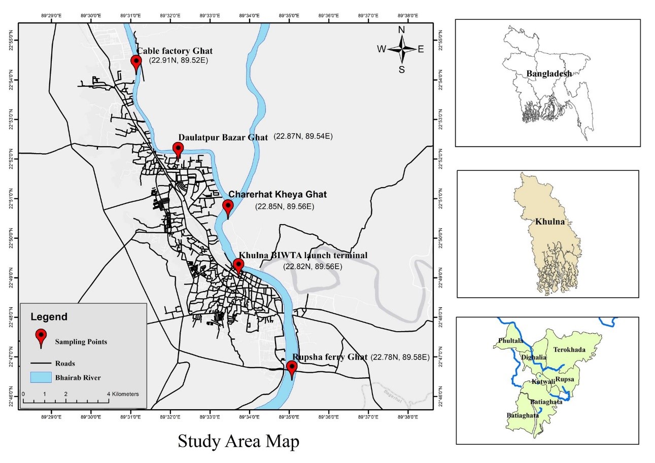
| Sampling ID | Sampling Station Name | Latitude | Longitude | Chainage in km (measured by Google Earth) | Remarks |
| 1 | Rupsha Ferry Ghat | 22° 46′ 48” N | 89° 34′ 48” E | 0.0 | The water collection points were chosen based on a sense of accessibility and a somewhat uniform interval. |
| 2 | Khulna BIWTA Launch Terminal | 22° 49′ 12” N | 89° 33′ 36” E | 4.88 | |
| 3 | Charerhat Kheya Ghat | 22° 51′ 0” N | 89° 33′ 36” E | 8.02 | |
| 4 | Daulatpur Bazar Ghat | 22° 52′ 12” N | 89° 32′ 24” E | 10.78 | |
| 5 | Cable Factory Ghat | 22° 54′ 36” N | 89° 31′ 12” E | 15.66 |
Description of the study area
The study was conducted on Bhairab river within Khulna region which is in the southwest of Bangladesh. The district of Khulna is located between 22°12′ and 23°59′ north latitudes and 89°14′ and 89°45′ east longitudes. The district’s total land area is 4389.11 square kilometres, of which 607.80 square kilometres are riverine (BBS, 2013). The region’s system of rivers plays a crucial part in its economy. All the major rivers of Khulna are attached to the Bay of Bengal via streams and canals. Along the city’s eastern border, the Bhairab on the northern side, the Rupsha River in the middle, and the Pasur on the southern side flow (Adhikari et al., 2006). The River Bhairab flows into the Rupsha at its terminus.
Methods of the Study
Sample collection
At five locations along the Bhairab River from upstream to downstream, water samples were taken during both high and low tides and sampling was carried out seasonally [the wet season (June, 2022) and the dry season (November, 2022)]. Sampling was conducted through more less uniform interval grab sampling technique to identify fluctuations in the flux of heavy metals in the river water. So altogether 30 samples were collected in each season considering the tidal condition of the river and sample replicates. As per the hydrological regime of the basin, the sampling seasons were chosen. The sampling stations are illustrated in Fig 2.1. In the field, decontaminated polypropylene bottles were used to collect a one-liter sample at a depth of approximately 50 centimetres below the river’s surface. There were three replicate samples gathered at each site. To collect water samples, one-liter polypropylene bottles were utilized. Prior to sample collection, all bottles were cleansed with river water to eliminate the possibility of contamination from extraneous components present in the bottles.
Sample treatment and preservation method
The water samples were digested and then transferred to designated plastic vials for analysis. 50 mL of each sample was digested with HNO3 according to the USEPA SW Method 3005 (USEPA 1987) procedure for the digestion of water sample: 50 ml of HNO3 was added to the sample in the beaker, which was then covered and heated in a fume cupboard using a hot plate until the volume was reduced to 15-20 mL. The samples were cooled and then filtered through Whatman No. 41 filter paper. It was then quantitatively transferred to a 50 mL volumetric flask and topped up with distilled water. In the course of the analysis, quality control methods and blanks were employed. Samples were evaluated alongside sample blanks and replicate samples to guarantee the precision and accuracy of the analyses. To prevent precipitation and adsorption on container walls, collected samples were acidified with pure nitric acid to a pH below 2.0. The samples were delivered to the laboratory for analysis after being maintained at 4ºC in an ice-container.
Methods for analysing water quality parameters
Water quality parameters were analysed both in field and laboratory.
Field investigation
The hydrogen ion concentration (pH), temperature and dissolved oxygen (DO) of the sample were determined in the field using proper instruments.
Temperature
Temperature is a crucial quality of water and ambient variable because it affects the rate of chemical and biological processes. TDS meter was used for recording temperature values in Degree Celsius unit of water sample (APHA, 1998).
Dissolved oxygen
Dissolved oxygen (DO) is among the most significant water quality parameters. Fish and other aquatic species require it to survive. Due to the aerating effect of wind, oxygen dissolves in surface water. Additionally, oxygen is released into the water as a consequence of photosynthesis in aquatic plants. DO (mg/l) meter was used for determination of dissolved oxygen concentration of the water sample.
Laboratory analysis
The pH, TDS, EC, COD, BOD, turbidity and concentration of selected metals for this study was analysed in the laboratory.
pH
Since hydrogen ion concentration of water can be altered by dissolved compounds, pH is a significant detector of chemical change in water. pH value of the sample water was directly measured through Hanna Bench Top pH Meter HI-2211 (APHA, 1998).
TDS
In water bodies such as rivers, higher concentrations of total dissolved solids are frequently detrimental to aquatic life. The TDS modifies the mineral content of the water, which is crucial to the maintenance of a variety of species. Additionally, dissolved salt can dry aquatic animal skin, which can be lethal. TDS Meter (HQ40D Portable Multi Meter) was used for measuring TDS (mg/l) of the water sample (APHA, 1998).
EC
The significance of water conductivity stems from the fact that it reveals the concentration of dissolved compounds, chemicals, and minerals. The content and nature of salt content alter the electro conductivity of a water sample. TDS Meter (HQ40D Portable Multi Meter) was used for measuring EC (uS/cm) and salinity (g/L) of the water sample (APHA, 1998).
BOD5
BOD5 was calculated after five days of sampling. The samples were stored in a black taped glass bottle to prevent the light. The DO was measured immediately after sampling and another reading of DO was taken after five days of sampling. The BOD value came out from deducting the second value of DO from the first. The method followed APHA (1998) guidelines.
COD
COD was measured using closed flux method guided by APHA 1998 guidelines.
Turbidity
The turbidity of a body of water is determined by shining a light through it and measuring the amount of scattered light. The unit for turbidity was in NTU. It followed the APHA (1998) rules.
Determination of selected metals in water sample
The concentration of selected metals (mg/l) in the sample water was estimated in the laboratory of JUST. Using atomic absorption spectrophotometer, Fe, Mn, Zn concentrations were determined. The concentration of arsenic was determined through HG-AAS (Hydride Generation Atomic Absorption Spectrophotometry) and Flame Atomic Absorption Spectroscopy method was used to determine the concentration of Cr, Cd, Ni, Pb and Cu. The analysis was conducted according to APHA (1998) and USEPA 3005 standard methods (USEPA, 1987).
Methods for data collection
Primary data
Laboratory experiments were conducted to get the values of the desired water quality parameters.
Secondary data
Secondary data was collected from guidelines of surface water quality parameters for various purposes published by WHO (2009), DOE (2002; 2005), Irrigation standard (Ayers and Westcot 1976), Bangladesh Standard for Fisheries (EQS,1997) and Domestic Standards (De, 2005).
Pollution assessment methods of heavy metals
Heavy metal pollution index (HPI)
The Heavy Metal Pollution Index (HPI) was utilized to evaluate water quality based on heavy metal concentration using MS Excel 2016.
The heavy metal pollution index (HPI) was calculated as follows (Mohan et al., 1996):
\[HPI= \sum_{i=1}^{n} \frac{Wi*Qi}{Wi} \tag{2.1}\]
Where Qi denotes the Sub index of the ith parameter, Wi indicates the unit weight of the ith parameter, and n stands for the number of determined parameters. The sub index (Qi) for every parameter was computed as follows:
\[HPI= \sum_{i}^{n} 100X (\frac{Mi-Li}{Si-Li}) \tag{2.2}\]
Where Mi indicated the assessed value of the ith heavy metal variable, Li represented the ideal value of the ith parameter, and Si indicated the standard value of the ith parameter.
Index of single-factor pollution
The single factor index approach was used to evaluate the level of contamination of a single pollutant in sediment samples (N. Yan et al., 2016). In the present study, this approach was utilized to determine the degree of contamination of one contaminant in river water samples using MS Excel 2016. This approach could identify the pollutant that contributes the most to pollution at each sampling location. The pollution index for a single pollutant was calculated using the formula:
\[Pi=\frac{Cn}{Sn} \tag{2.3}\]
Where Pi is the single factor pollution index, Cn (mg/L) is the measured concentration of heavy metals, and Sn (mg/L) is the pollutant standard value. The single factor index’s value Pi 1 denotes clean pollution levels, 1< Pi ≤ 2 is considered low pollution levels, 2 < Pi≤ 3 is considered moderate, and Pi> 3 indicates high pollution levels (N. Yan et al., 2016; Liu, M. et al., 2018).
Multivariate statistical analysis
Pearson’s correlation matrix was utilized to represent the relationship between the pairs of variables. The correlation coefficient matrix measures the extent to which the variance of each component may be explained by their relationship (C-W. Liu et al., 2003). In this work, experimental river water data were statistically analysed using IBM SPSS software (version 25).
RESULTS AND DISCUSSION
Analysis of the Physicochemical Properties of River Water
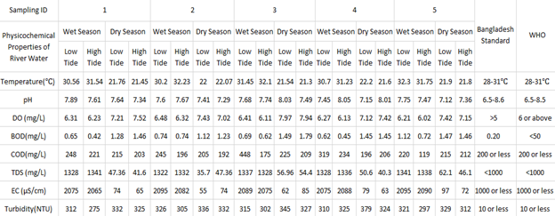
Findings of the physicochemical parameters of water samples studied during the wet (June, 2022) and dry (November, 2022) seasons are shown in Table 3.1. The parameters were compared with Bangladesh Standards (DOE, 2001; 2005), Bangladesh Standard for Fisheries (EQS,1997), Domestic Standards (De, 2005), Drinking Standards (ADB ,1994) and Irrigation standard (Ayers and Westcot 1976).
Statistical representation of physicochemical parameters of river water
This attention of this study was specifically drawn to certain physicochemical characteristics of the Bhairab River, including temperature, turbidity, conductivity or electric conductivity, dissolved oxygen, chemical oxygen demand, biological oxygen demand, pH and total dissolved solids.
The parameters are assessed in wet and dry seasons during high and low tide to avoid any negligence towards the variance in the output in terms of weather or tidal flow. The minimum, maximum and mean values were calculated for the comparison with national and international water quality parameter standards.
| Parameters | Wet Season | Dry Season | ||||||||||
| Low Tide | High Tide | Low Tide | High tide | |||||||||
| Min | Max | Mean | Min | Max | Mean | Min | Max | Mean | Min | Max | Mean | |
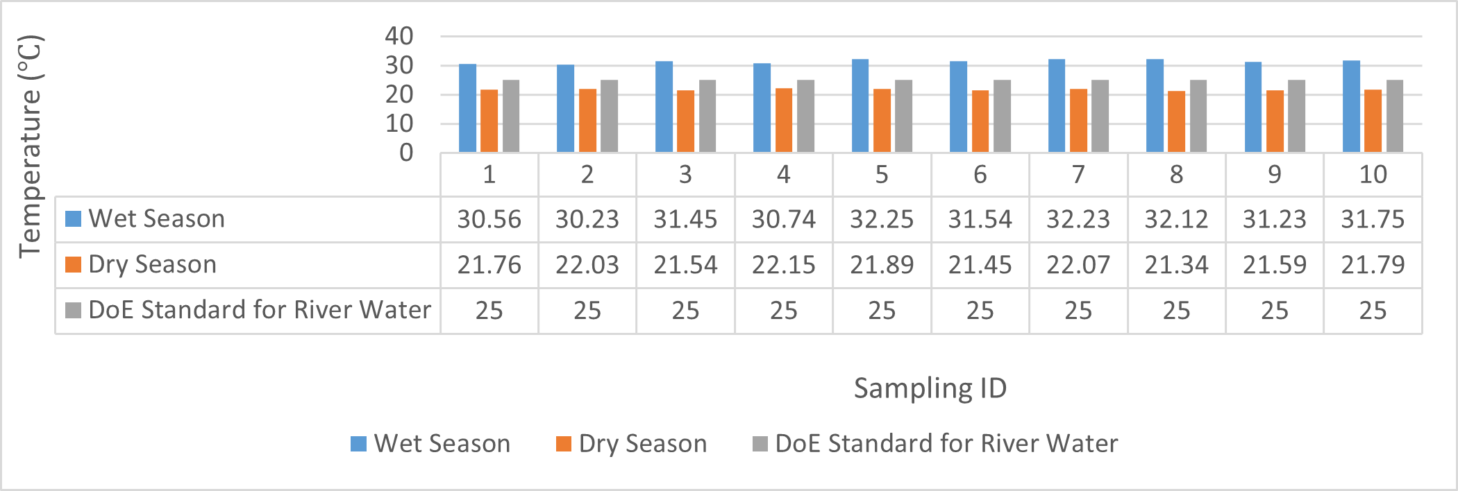
| Temperature(℃) | 30.23 | 32.25 | 31.046 | 31.23 | 32.23 | 31.774 | 21.54 | 22.15 | 21.874 | 21.34 | 22.07 | 21.648 |
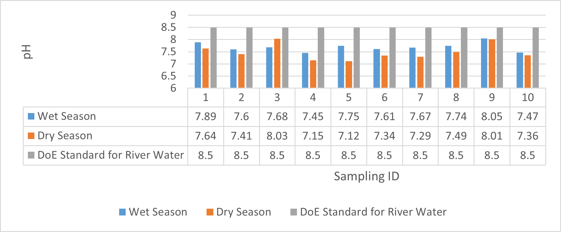
| pH | 7.45 | 7.89 | 7.674 | 7.47 | 8.05 | 7.708 | 7.12 | 8.03 | 7.47 | 7.29 | 8.01 | 7.498 |
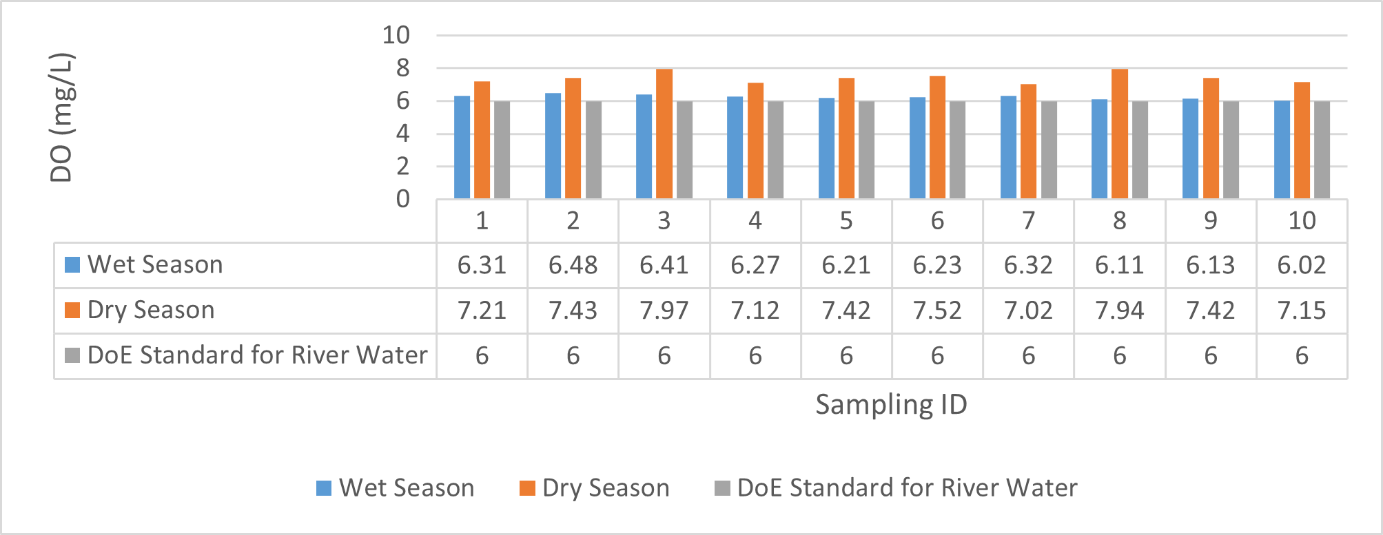
| DO (mg/L) | 6.21 | 6.48 | 6.336 | 6.02 | 6.32 | 6.162 | 7.12 | 7.97 | 7.43 | 7.02 | 7.94 | 7.41 |
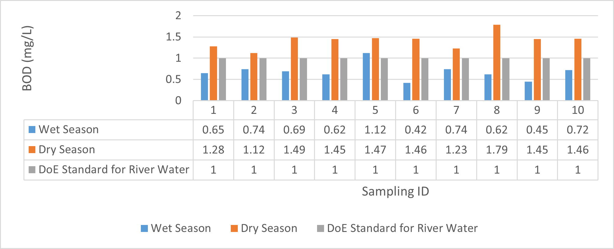
| BOD(mg/L) | 0.62 | 1.12 | 0.764 | 0.42 | 0.74 | 0.59 | 1.12 | 1.49 | 1.362 | 1.23 | 1.79 | 1.478 |
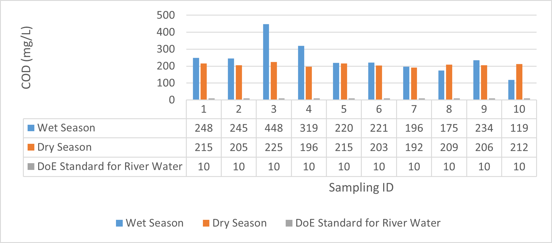
| COD(mg/L) | 220 | 448 | 296 | 119 | 234 | 189 | 196 | 225 | 211.2 | 192 | 212 | 204.4 |
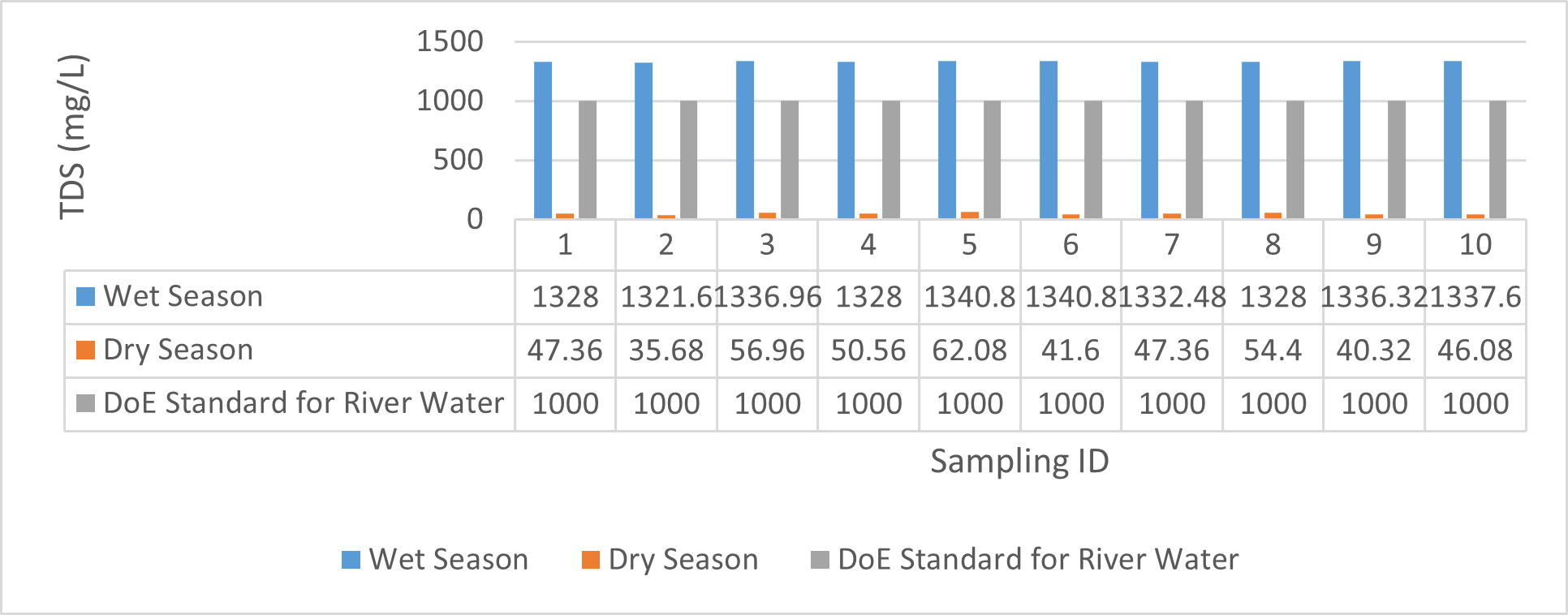
| TDS (mg/L) | 1321.6 | 1340.8 | 1331.07 | 1328 | 1340.8 | 1335.04 | 35.68 | 62.08 | 50.528 | 40.32 | 54.4 | 45.952 |
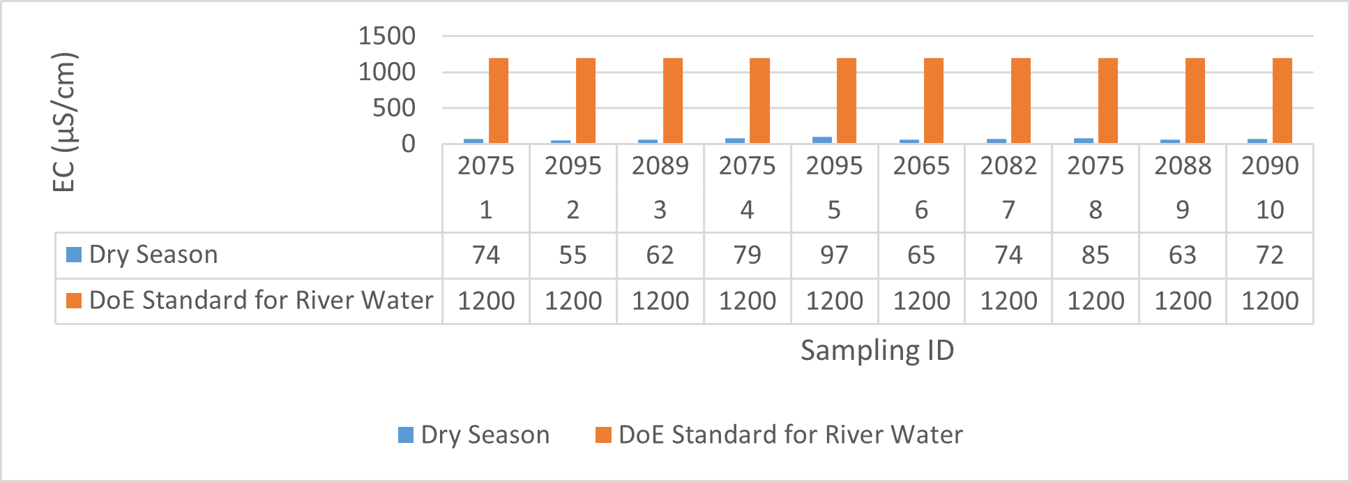
| EC (μS/cm) | 2075 | 2095 | 2085.8 | 2065 | 2090 | 2080 | 55 | 97 | 73.4 | 63 | 85 | 71.8 |
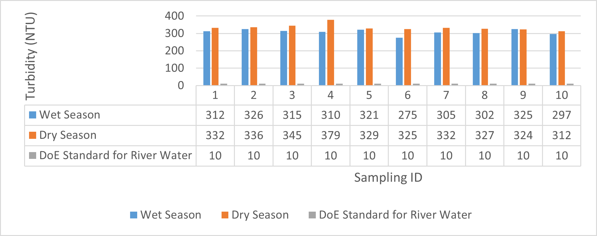
| Turbidity
(NTU) |
310 | 326 | 316.8 | 275 | 325 | 300.8 | 329 | 379 | 344.2 | 312 | 332 | 324 |
Analysis of water quality for different purpose based on measured physicochemical parameters of water samples
Findings on physicochemical properties of Bhairab river, Khulna, was presented in Table 3.1. The minimum, maximum and mean values were presented in Table 3.2. During wet season, temperature ranges from 30.23ºC-32.25ºC and the mean value is 31.41ºC. On the other hand, temperature ranges from 21.34ºC-22.15ºC and the mean value is 21.76ºC in dry season. WHO (2011) standard for drinking water recommends 12ºC -25ºC as the suitable range. The temperature mean of dry season can be acknowledged as suitable for drinking, irrigation and fish culture in terms of temperature. DOE (2005) suggests 20ºC-30ºC as suitable temperature range for both drinking and irrigation. The Bangladesh Fisheries Standard (EQS, 1997) had set the suitable temperature 25ºC for fish culture. The mean value of pH came out as 7.69 ranging from 7.45 to 8.05 during wet season and the pH value ranges from 7.12 to 8.03 and the mean value is 7.48 during dry season. So the pH value is higher during wet season. In accordance with the recommended Bangladesh Standards and Bangladesh Environment Conservation Rule (ECR), the pH range for irrigation water is between 6.50 and 8. (DOE, 2005; ECR, 1997). According to Ayers and Westcot (1985), the recommended pH range for irrigation water is between 6.5 and 8.4. WHO (2011) recommended value of pH for drinking water as 6.5-8.5 and The Bangladesh Fisheries Standard (EQS, 1997) also recommended the similar range of pH for fish culture. So the water is suitable for irrigation, drinking and fish culture in both seasons judging from the mean value of pH. Dissolved oxygen ranged from 6.02 to 6.48 (mean value was 6.249) during wet season and 7.02-7.97 during dry season (mean value was 7.42). DOE (2005), Fisheries (EQR, 1997) and Domestic Supply (De, 2005) standard suggests 6.5, 4-6 and 4-6 mg/L as the optimum level for DO (Dissolved oxygen). DO is observed 7.4 mg/L during dry season and 6.1-6.3 mg/L as the mean values. So DO indicates that the river water has optimum level of DO for fish culture and domestic water supply in dry season but it exceeded the range during wet season. The desired level for turbidity according to Bangladesh Standard (ECR, 1997) is 10 NTU. So both season exceeded the optimum level for turbidity (mean value of turbidity was 308 during wet season and 334 NTU during dry season). BOD range during wet season was 0.5-0.7mg/L (mean value) and dry season was 1.3-1.4 mg/L (mean value). DOE (2005) standard for river water is 5 mg/L and (-) or less than 2 mg/L is accurate for drinking, less than 6mg/L for fish culture (EQR, 1997) and 0-10mg/L for irrigation (Ayers and Westcot, 1985). So the BOD level is within the standard range for fish culture and irrigation according to the mean value (0.6mg/L in wet season and 1.42 mg/L in dry season). The COD is 189 mg/L during high tide and 296 mg/L during low tide as the mean values in wet season. On the other hand, the value was recorded as 211 mg/L (low tide), 204 mg/L (high tide) in dry season. The recommended value for COD is 200 or less according to Bangladesh Standard. The COD level seemingly exceeded the optimum value during dry season but it is within the range during low tide of wet season.
Evaluation of Heavy Metal Pollution in the Bhairab River Water
The concentration of selected metal including Arsenic (As), Iron (Fe), Manganese (Mn), Lead (Pb), Chromium (Cr), Cadmium (Cd), Nickel (Ni), Copper (Cu) and Zinc (Zn) were determined and compared with WHO (2009) and Bangladesh Guideline for river water quality for assessing the suitability of river water in terms of various purposes such as, drinking water supply, irrigation, fish culture etc. The pollution caused by selected metals was analyzed using Heavy Metal Pollution Index (Mohan et al., 1996). There, if the 100 is the reference value to determine the pollution in the river water caused by metals. If the value came out as less than 100 then it was considered that the river water is safe for drinking and free from heavy metal pollution but if the value was higher than 100, it was considered otherwise. Single Factor Pollution Index approach provided a fair estimate of an individual heavy metal contamination in water samples. The distribution pattern of contamination by heavy metals in sampling locations is depicted in Fig 3.20 to Fig 3.37 using the Pi value as the output of the single factor pollution indexing method.
Concentration of assessed metals in river water
Concentration calculated at each sampling station during high and low tide in wet season is depicted in Table 3.3 and Table 3.4 shows the concentration recorded during dry season. The minimum and maximum value were calculated to analyze the range and the mean value was calculated as well.
| Low Tide | |||||||||
| Sampling ID | As(mg/L) | Mn (mg/L) | Fe(mg/L) | Pb (mg/L) | Cu(mg/L) | Zn(mg/L) | Cr(mg/L) | Cd(mg/L) | Ni(mg/L) |
| 1 | 0.01 | 0.12 | 2.32 | 0.1 | 0.0689 | 0.09 | 0.04 | 0.0347 | 0.0051 |
| 2 | 0.009 | 0.16 | 2.25 | 0.07 | 0.2497 | 0.1 | 0.1 | 0.0482 | 0.0068 |
| 3 | 0.006 | 0.1 | 2.42 | 0.09 | 0.3531 | 0.95 | 0.1 | 0.0579 | 0.0063 |
| 4 | 0.012 | 0.13 | 2.43 | 0.1 | 0.1679 | 0.82 | 0.12 | 0.0733 | 0.0066 |
| 5 | 0.011 | 0.12 | 2.3 | 0.09 | 0.211 | 0.1 | 0.17 | 0.0511 | 0.0063 |
| Min | 0.006 | 0.1 | 2.25 | 0.07 | 0.0689 | 0.09 | 0.04 | 0.0347 | 0.0051 |
| Max | 0.012 | 0.16 | 2.43 | 0.1 | 0.3531 | 0.95 | 0.17 | 0.0733 | 0.0068 |
| Mean | 0.0096 | 0.126 | 2.344 | 0.09 | 0.21012 | 0.412 | 0.106 | 0.05304 | 0.00622 |
| SD | 0.002302 | 0.021909 | 0.078294 | 0.012247 | 0.104566 | 0.434246 | 0.04669 | 0.014121 | 0.000661 |
| High Tide | |||||||||
| 6 | 0.007 | 0.11 | 2.22 | 0.1 | 0.5468 | 0.91 | 0.01 | 0.0489 | 0.0059 |
| 7 | 0.014 | 0.14 | 2.41 | 0.1 | 0.4478 | 0.08 | 0.08 | 0.0619 | 0.0067 |
| 8 | 0.021 | 0.13 | 2.27 | 0.09 | 0.1378 | 0.1 | 0.07 | 0.0639 | 0.0053 |
| 9 | 0.015 | 0.12 | 2.34 | 0.1 | 0.1335 | 0.91 | 0.11 | 0.0755 | 0.0055 |
| 10 | 0.013 | 0.11 | 2.38 | 0.09 | 0.1464 | 0.07 | 0.17 | 0.0809 | 0.0059 |
| Min | 0.007 | 0.11 | 2.22 | 0.09 | 0.1335 | 0.07 | 0.01 | 0.0489 | 0.0053 |
| Max | 0.021 | 0.14 | 2.41 | 0.1 | 0.5468 | 0.91 | 0.17 | 0.0809 | 0.0067 |
| Mean | 0.014 | 0.122 | 2.324 | 0.096 | 0.28246 | 0.414 | 0.088 | 0.06622 | 0.00586 |
| SD | 0.005 | 0.013038 | 0.078294 | 0.005477 | 0.199274 | 0.452913 | 0.058481 | 0.012506 | 0.000537 |
| Low Tide | |||||||||
| Sample ID | As(mg/L) | Mn(mg/L) | Fe(mg/L) | Pb(mg/L) | Cu(mg/L) | Zn(mg/L) | Cr(mg/L) | Cd(mg/L) | Ni(mg/L) |
| 1 | 0.013 | 0.04 | 3.32 | 0.082 | 0.23 | 0.08 | 0.0374 | 0.0062 | 0.186 |
| 2 | 0.017 | 0.03 | 3.24 | 0.28 | 0.43 | 0.12 | 0.0497 | 0.0089 | 0.1 |
| 3 | 0.011 | 0.06 | 3.31 | 0.36 | 0.77 | 0.11 | 0.0593 | 0.01 | 0.12 |
| 4 | 0.015 | 0.02 | 3.59 | 0.171 | 0.67 | 0.15 | 0.0769 | 0.012 | 0.167 |
| 5 | 0.016 | 0.04 | 3.26 | 0.215 | 0.75 | 0.19 | 0.0575 | 0.0093 | 0.2 |
| Min | 0.011 | 0.02 | 3.24 | 0.082 | 0.23 | 0.08 | 0.0374 | 0.0062 | 0.1 |
| Max | 0.017 | 0.06 | 3.59 | 0.36 | 0.77 | 0.19 | 0.0769 | 0.012 | 0.2 |
| Mean | 0.0144 | 0.038 | 3.344 | 0.2216 | 0.57 | 0.13 | 0.05616 | 0.00928 | 0.1546 |
| SD | 0.002408 | 0.014832 | 0.141527 | 0.105661 | 0.233238 | 0.041833 | 0.014452 | 0.002095 | 0.042951 |
| High Tide | |||||||||
| 6 | 0.013 | 0.05 | 3.28 | 0.552 | 0.39 | 0.04 | 0.05 | 0.0098 | 0.159 |
| 7 | 0.014 | 0.03 | 3.52 | 0.45 | 0.1 | 0.13 | 0.0684 | 0.0087 | 0.174 |
| 8 | 0.016 | 0.04 | 3.23 | 0.14 | 0.38 | 0.15 | 0.0694 | 0.0084 | 0.192 |
| 9 | 0.019 | 0.06 | 3.39 | 0.137 | 0.42 | 0.16 | 0.0791 | 0.0081 | 0.164 |
| 10 | 0.012 | 0.03 | 3.21 | 0.148 | 0.33 | 0.23 | 0.0821 | 0.00732 | 0.188 |
| Min | 0.012 | 0.03 | 3.21 | 0.137 | 0.1 | 0.04 | 0.05 | 0.00732 | 0.159 |
| Max | 0.019 | 0.06 | 3.52 | 0.552 | 0.42 | 0.23 | 0.0821 | 0.0098 | 0.192 |
| Mean | 0.0148 | 0.042 | 3.326 | 0.2854 | 0.324 | 0.142 | 0.0698 | 0.008464 | 0.1754 |
| SD | 0.002775 | 0.013038 | 0.128957 | 0.200132 | 0.129345 | 0.068337 | 0.012569 | 0.000906 | 0.01445 |
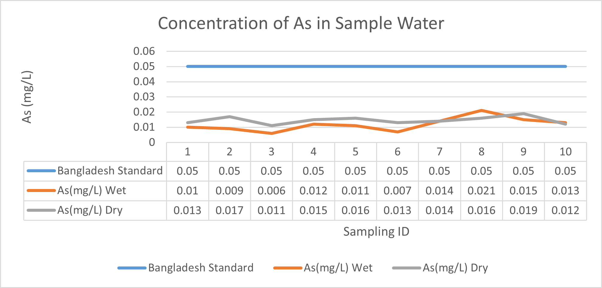
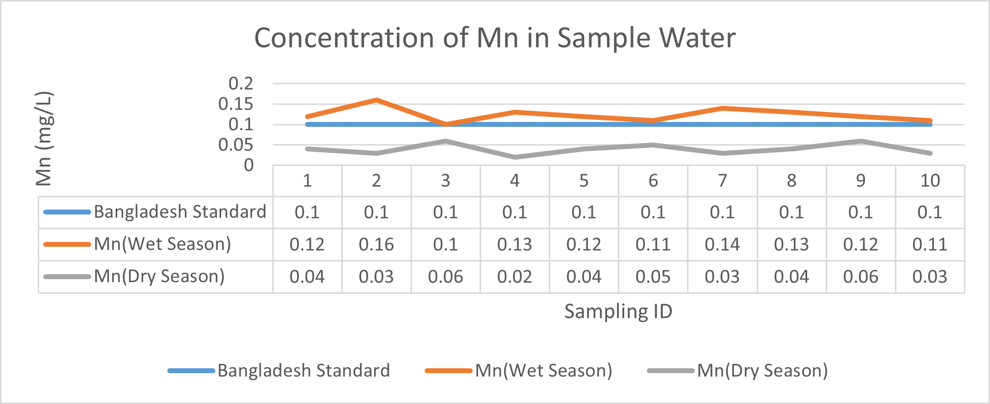
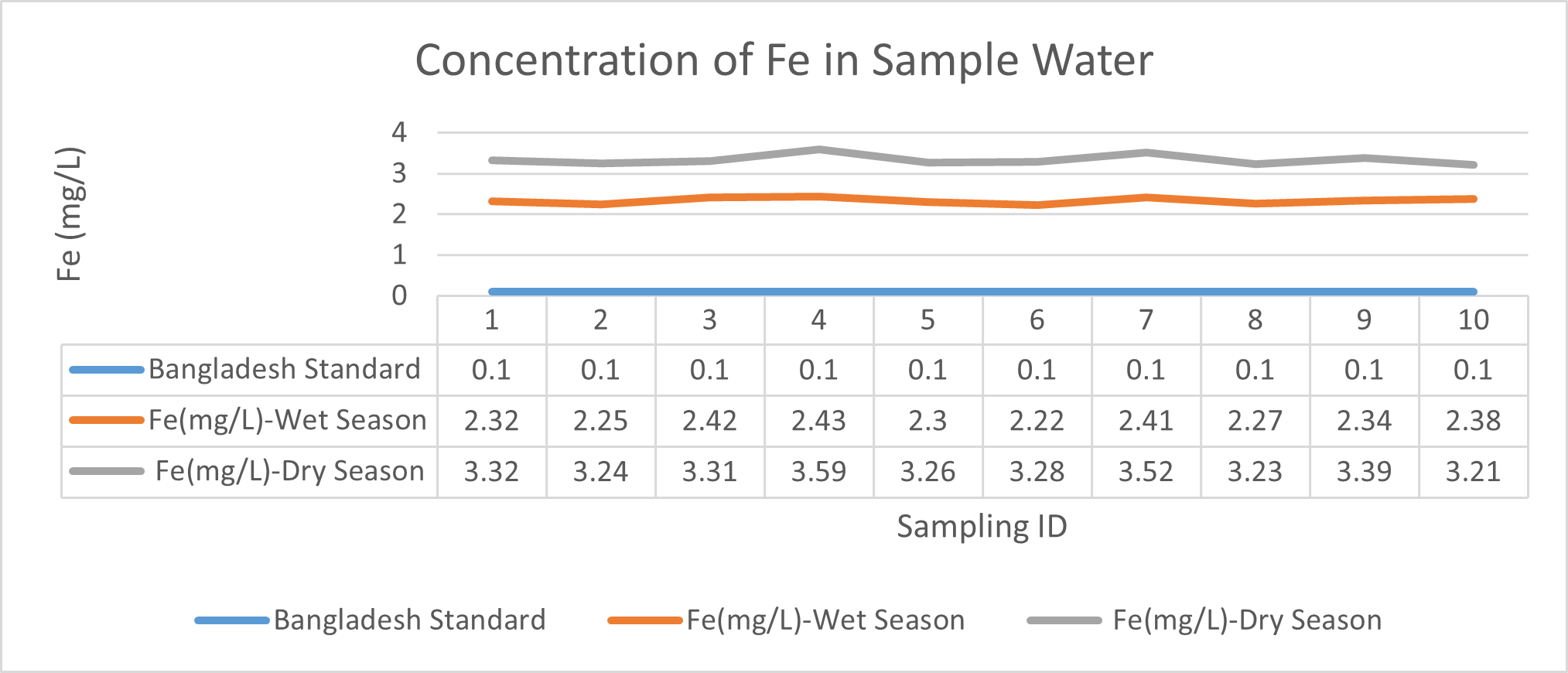
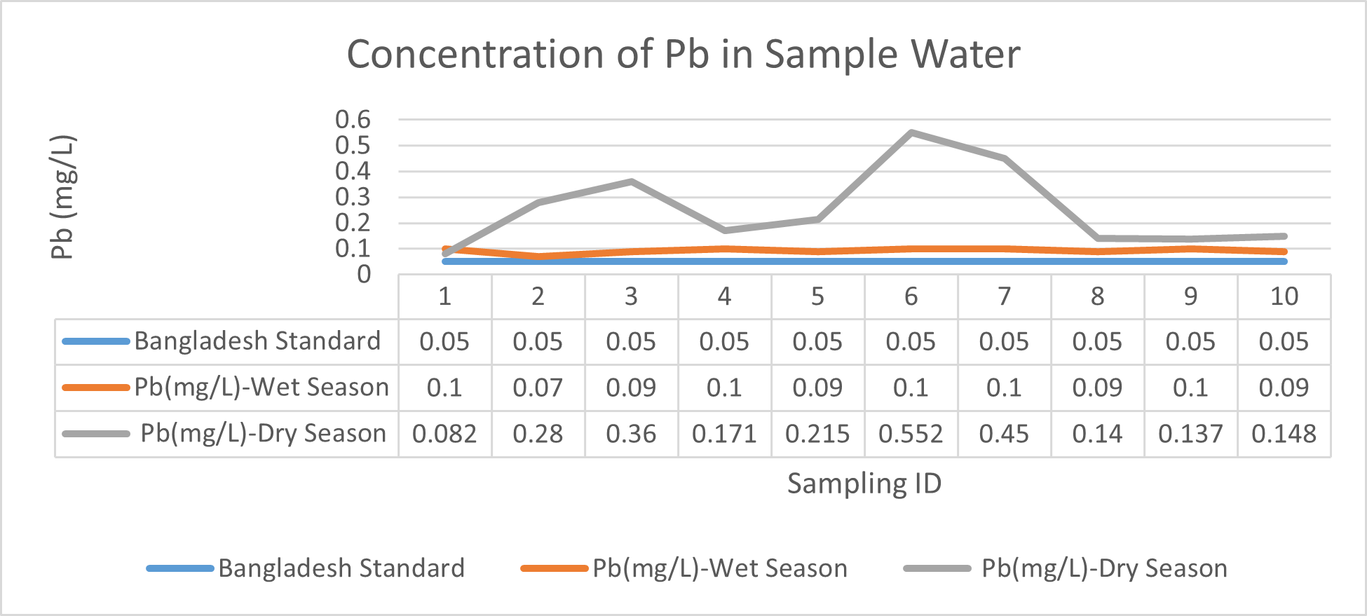
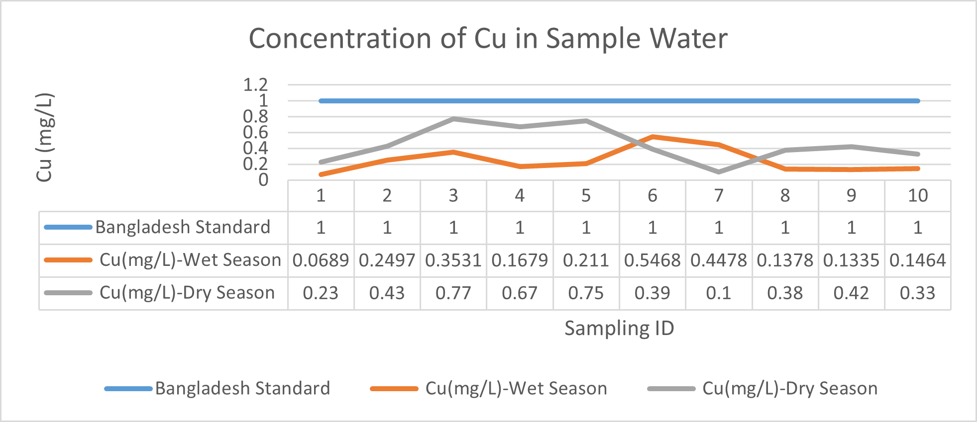
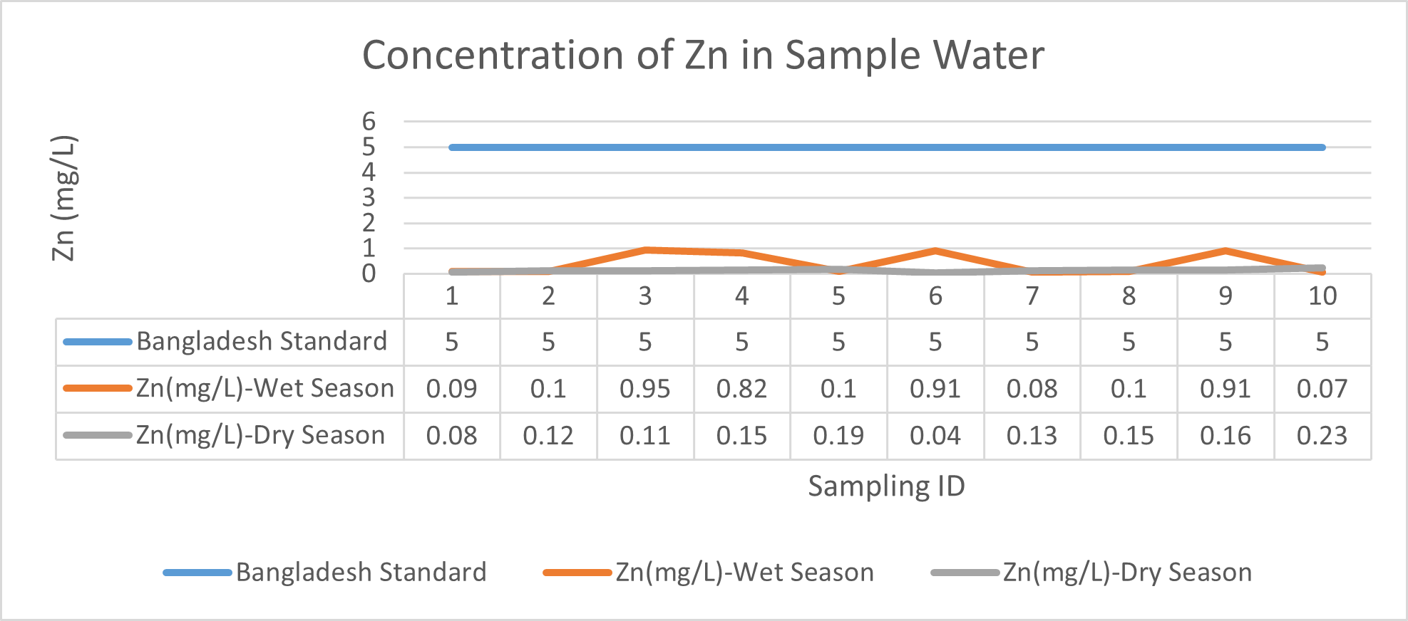
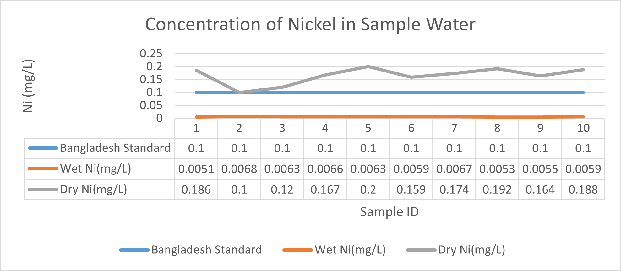
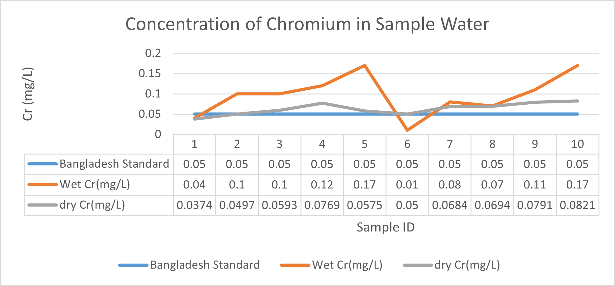
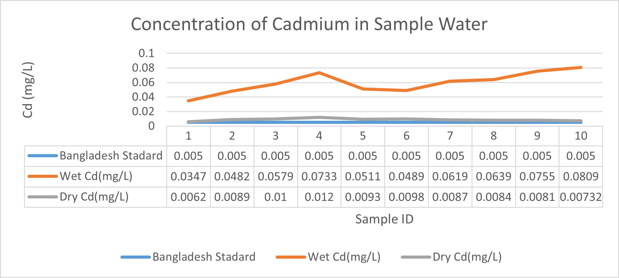
Arsenic ranges from 0.011mg/L to 0.019mg/L with a mean value of 0.014mg/L during dry season and 0.006mg/L-0.021mg/L with a mean value of 0.0118mg/L in dry season. So it seems that concentration of arsenic is less in wet season than that of dry season. Mean concentration of arsenic was within the optimum value proposed by WHO and Bangladesh Standard (0.05 mg/L). Mean concentration of manganese, zinc, nickel and copper was also observed to be within acceptable range. Copper ranges from 0.1mg/L to 0.7mg/L with a mean value of 0.4mg/L during dry season and 0.06mg/L to 0.5mg/L with a mean value of 0.2mg/L in wet season. So it seems that concentration of copper is less in wet season than that of dry season. Manganese ranges from 0.02mg/L to 0.06mg/L with a mean value of 0.04mg/L during dry season and 0.1mg/L to 0.16mg/L with a mean value of 0.124mg/L in wet season. So it seems that concentration of manganese is less in dry season than that of wet season. According to Ayers and Westcot (1985), the maximum amount of manganese permitted in irrigation water is 0.20 mg/L. Besides Ayers and Westcot (1985) stated that water with less than 0.20 mg/L copper is safe for irrigation. Similarly, the National Academy of Sciences has suggested that irrigation effluent water for prolonged usage should contain no more than 0.20 mg L-1 Cu (Gibeault and Cockerham, 1985). Maximum allowed Zn concentration in irrigation water is 2.0 mg/L (Ayers and Westcot, 1985). The mean concentration of zinc was 0.1mg/L during dry season and 0.4mg/L during wet season. So it came within the acceptable range for irrigation. However, iron concentration was much higher than the optimum value. Iron ranges from 3.21mg/L to 3.59mg/L with a mean value of 3.33mg/L during dry season and 2.22mg/L to 2.43mg/L with a mean value of 2.33mg/L in wet season. So it seems that concentration of iron is less in wet season than that of dry season. Bangladesh Standard guideline suggested that optimum value for lead should be 0.05 mg/L but the mean value is much higher during dry season (approximately 0.2 mg/L). Lead ranges from 0.08mg/L to 0.5mg/L with a mean value of 0.2mg/L during dry season and 0.07mg/L to 0.1mg/L with a mean value of 0.1mg/L in wet season. So it seems that concentration of lead is less in wet season than that of dry season. The threshold level for lead in household water supply, according to ISI (De, 2005), is 0.01 mg/L. Likewise, according to the Proposed Bangladesh Standards, the maximum lead concentration for irrigation water is 0.01 mg/L (DOE, 2005). On the other hand, cadmium showed higher concentration during wet season (approximately 0.05 mg/L) whereas the optimum value was 0.005 mg/L. But Ayers and Westcot indicated that water with less than 0.01 mg/L of cadmium is alright for irrigation (1985). The mean concentration of chromium was 0.06 mg/L during dry season and 0.09 mg/L during wet season which is slightly higher than recommended concentration (0.05 mg/L). Ayers and Westcot (1985) state that water with less than 0.20 mg L-1 of Cr is suitable for irrigation. The standard limit for Cu, Zn, Pb, Cd is 1mg/L, 5mg/L, 0.05mg/L, 0.005mg/L respectively in terms of drinking water (ADB, 2003). So from the analysis, we can say that although the river water might not be suitable for drinking but it is suitable for irrigation purposes as it passes the recommended level of heavy metals for irrigation water proposed by FAO. As for fish culture the standard concentrations of Cu, Zn, Pb, Fe and Cd are 0.03, <0.005, <0.02, <0.1 and 0.005mg/L respectively (EQR, 1997). So it can be seen that the water is suitable for fish culture in terms of copper and zinc concentration but it exceeds the ideal concentration of lead, iron and cadmium. From Fig 3.9 to Fig 3.17, it can be summarized that the concentration of As, Fe, Pb, Cu and Ni is higher dry season whereas Mn, Zn, Cr and Cd concentration is higher in wet season. The amount of heavy metals in water samples examined in the research region rises in the order of Fe > Cu > Pb > Ni > Cr > Mn > Zn > As > Cd during dry season and Fe > Zn > Cu > Mn > Cr > Pb > Cd > As > Ni during wet season.
Assessment of pollution level of river water using heavy metal pollution index
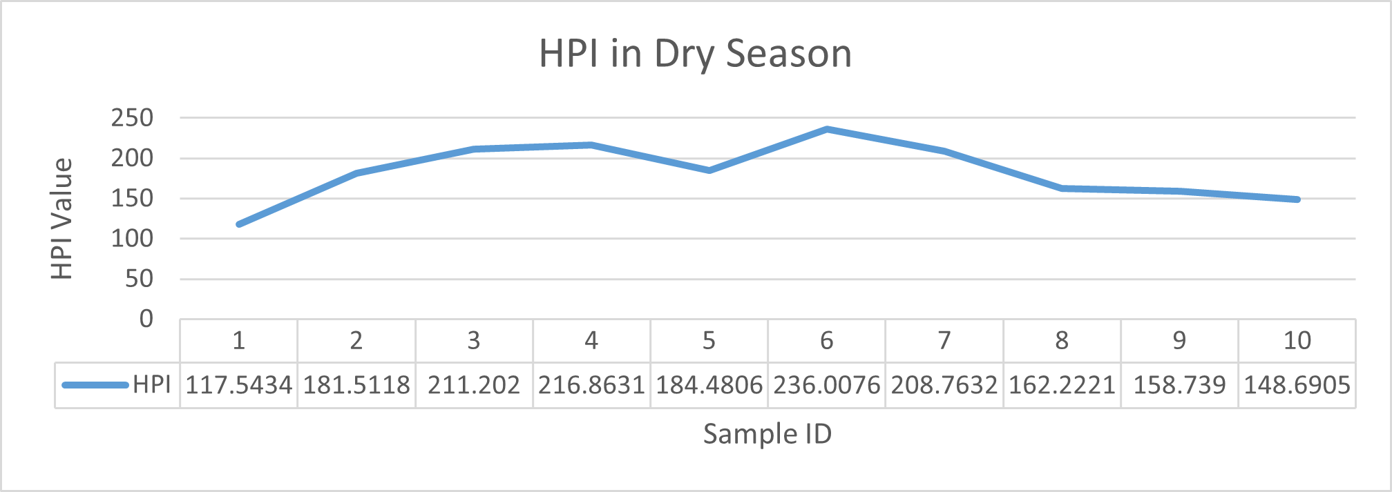
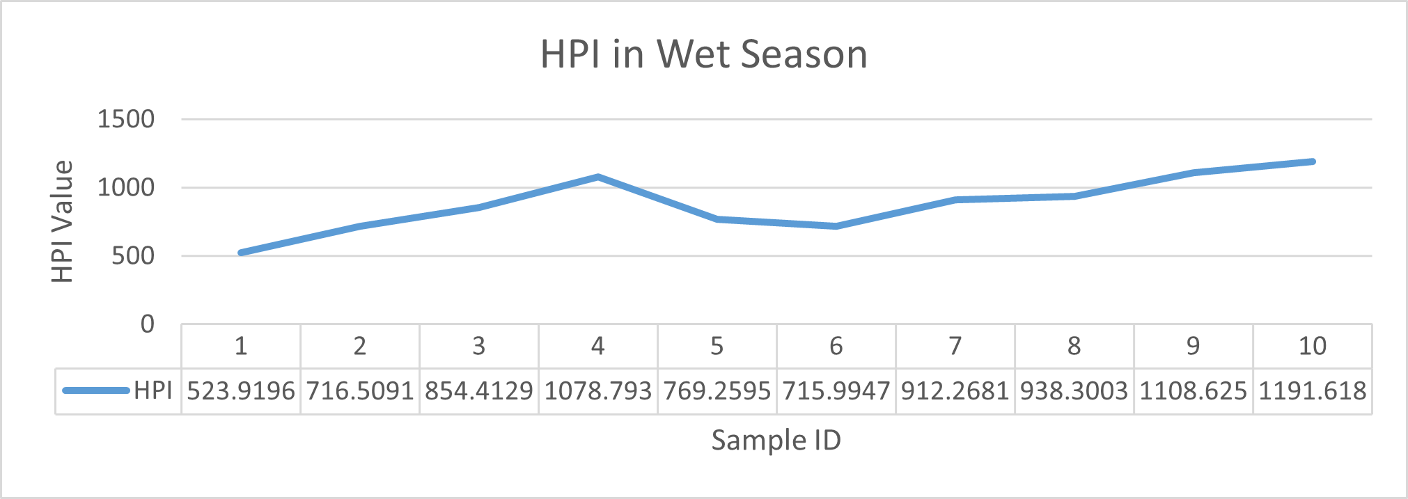
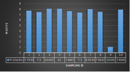
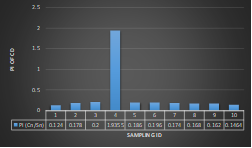
HPI indicates major pollution in river water during wet season although the value came out much lesser in dry season. The highest value was observed in wet season at sampling station 5 (Cable factory ghat) during high tides and lowest value was observed at station 1(Rupsha ferry ghat) in dry season during low tides. Table 3.5 shows the HPI of each site and status of pollution due to heavy metals available in that region whereas Fig 3.18 and Fig 3.19 depicts the statistical trend during dry and wet season respectively. As all the values came out greater than 100, it could be said that the river is having major pollution by the combined effect of the metals of interest (Mohan et al.,1996).
| Sampling Station No. | Season | Tide | HPI | Remarks |
| 1 | Dry Season | Low Tide | 117.5434 | Polluted by heavy metals, not safe for drinking purpose |
| High Tide | 236.0076 | |||
| 2 | Low Tide | 181.5118 | ||
| High Tide | 208.7632 | |||
| 3 | Low Tide | 211.202 | ||
| High Tide | 162.2221 | |||
| 4 | Low Tide | 216.8631 | ||
| High Tide | 158.739 | |||
| 5 | Low Tide | 184.4806 | ||
| High Tide | 148.6905 | |||
| 1 | Wet Season | Low Tide | 523.9196 | |
| High Tide | 715.9947 | |||
| 2 | Low Tide | 716.5091 | ||
| High Tide | 912.2681 | |||
| 3 | Low Tide | 854.4129 | ||
| High Tide | 938.3003 | |||
| 4 | Low Tide | 1078.793 | ||
| High Tide | 1108.625 | |||
| 5 | Low Tide | 769.2595 | ||
| High Tide | 1191.618 |
Estimation of the heavy metal contamination at each station
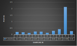
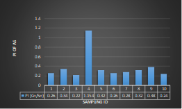
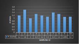
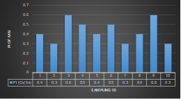
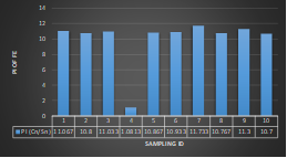
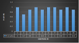
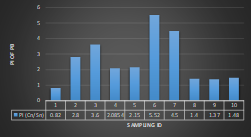
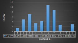
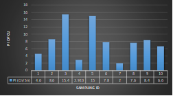
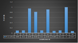
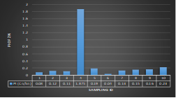
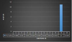
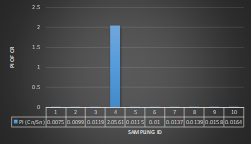
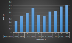
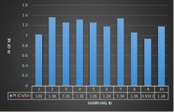
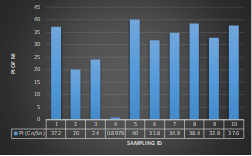
Here, in terms of arsenic concentration, sampling station 4 (Daulatpur Bazar Ghat) can be denoted as moderately polluted zone as the PI value was less than 2.5 (1.15 during wet season and 2.4 during dry season). Manganese seemed to be moderately affecting the clarity of river water quality in as the PI value is less than 2.5 but higher than 1(BIWTA Launch Terminal during low tide of wet season and Cable Factory Ghat during high tide of dry season). In terms of iron, it severely polluted all station except Daulatpur Bazar Ghat. Lead moderately polluted all sampling station during wet season but severely polluted in dry season. Cu severely polluted all sapling stations except Daulatpur Bazar Ghat during wet season, and all staions but Charerhat during dry season. Zinc polluted the river in moderate range during both seasons. Chromium seemed to pollute sampling station four in the moderate range during both seasons. Nickel affected the river water moderately during wet season but severely in dry season but exception went for Daulatpur Bazar Ghat during low tide of dry season.
Correlation Among Water Quality Parameters
The relation and interdependence among different variables were shown through Pearson’s Correlation Coefficient matrix are shown in Table 3.6 (wet season) and Table 3.7 (dry season). The blue colored cells show positive correlation and green colored cells show negative correlation. Correlation refers to the relationship between two independent variables. When a rise or reduction in the value of one variable corresponds to an increase or decrease in the value of the other, a direct link emerges. Positive correlation exists when a rise in one parameter leads to an increase in the other parameter, while negative correlation exists when an increase in one parameter leads to a drop in the other parameter. The correlation coefficient (r) ranges from +1 to -1. The correlation between the parameters is classified as strong when it falls within the interval 0.8 to 1.0, moderate when it falls within the interval 0.5 to 0.8, and weak when it falls within the interval 0.0.
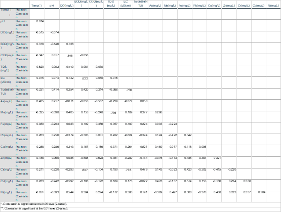
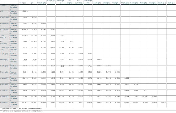
The p value represents the significance level of the correlation matrix. Additionally, it represents the intensity of relationships between heavy metals. p values of 0.01 and 0.05, for example, show strong and significant associations, respectively. The high positive association may indicate that heavy metals in diverse water samples originate from a same source (Dey, M. et al., 2021). Here Cu, Cd had strong significant positive correlation (r=.642) meaning that they might have similar source. Temperature, DO, BOD and Mn showed strong significant negative correlation (r=.763, .685, .747 respectively). Fe and COD showed strong significant negative correlation (r=.649). Fe, Cd and Turbidity showed strong significant positive correlation.
Discussion on the Surroundings of Sampling Stations
Table 3.8 shows the surrounding locality of the sampling stations and its contribution to river water quality degradation.
| Sampling ID | Sampling Station | Surrounding Locality |
| 1 | Rupsha Ferry Ghat | Khulna Printing and Packaging (Printing Industry), Sundarban sea food industries ltd, Modern Sea Food Industries ltd, Shahnewaz Seafood, Bangladesh seafood (sea food industry), Chor Rupsha Bazar (Market), Challenger Ice, Sun Shing Cement Mills (Cement Factory), Orion Power ltd (Power Station) etc
|
| 2 | BIWTA Launch Terminal | Khulna Sadar Hospital, Baro Bazar, The Wave Cruise Ship (Shipping Service) etc. |
| 3 | Charerhat Kheya Ghat | Khalishpur Jute Mills, Khulna Newsprint Mill, Khulna Jetty of Mongla Port etc |
| 4 | Daulatpur Bazar Ghat | Daulatpur Market, Crop Field, Khulna BSCIC |
| 5 | Cable Factory Ghat | BRR Cable Industries ltd |
Industries generate enormous quantities of garbage such as lead (mostly from the battery sector), which contains hazardous compound and damages environment. Many industries lack a proper waste management system, which results in the discharge of garbage into the waterway. Sea food industries exhibit high amount of metalloid pollutants and other hazardous compound as they directly discharge their effluent to the river. Although some industries have ETP but they do not function enough to eradicate all the hazardous compound in the effluent from industrial activity. Thus it leads to the availability of lead, cadmium, nickel, chromium etc. Sewage, accidental oil spill from launches, ships may cause increase in pollutant content. Urban runoff, agricultural runoff from hazardous chemical fertilizer applied crop field may result in increase of heavy metals in river water.
CONCLUSION
The Bhairab River is the only perennial surface water source within the basin that replenishes the shallow aquifers utilized for agriculture and residential purposes. During the year 2022, a number of significant water quality indicators, including Temperature, pH, Turbidity, Conductivity, EC, TDS, DO, BOD, COD, Manganese, Nickel, Zinc, Copper, Chromium, Cadmium, Arsenic, Iron, and Lead, were examined. The physiochemical parameters (temperature, pH, DO, BOD, TDS) of the region’s water samples (temperature, pH, DO, BOD, TDS) were within the Bangladesh Standards and WHO allowable limits for potable water. But COD, EC, and turbidity were not within the optimal range for potable water. There was a seasonal effect on the physiochemical parameters of drinking water in the region, with greater values obtained during the rainy season for temperature, pH, COD, and TDS, compared to the dry season for EC, turbidity, BOD, and DO. Except for arsenic, copper, and zinc, whose concentrations were below the optimum range, the concentration of heavy metals in the water surpassed WHO and Bangladesh guidelines. During the dry season, the concentration of heavy metals in water increases as follows: Fe > Cu > Pb > Ni > Cr > Mn > Zn > As > Cd; during the rainy season, the order is Fe > Zn > Cu > Mn > Pb > Ni > Cr > As > Cd. It was hypothesized that effluents were emitted by the print and electronic sectors, as well as from irrigation and domestic wastes, with a minimal contribution from geogenic sources. The majority of the metals surpassed the guidelines’ permitted limit. The average HPI measured throughout the study for both seasons was greater than 100, making the water undrinkable. The country sees great variation in water availability during floods during the monsoon season (June to October) and droughts during the dry season (November to May), which contributes to a severe incursion of salt into the interior. Bangladesh is a nation that has struggled with these problems throughout its brief history. Now, as a result of the intensifying effects of climate change, these obstacles are intensifying as the temperature rises and water variability grows.
REFERENCES
Adhikari, D. K., Roy, M. K., Datta, D. K., Roy, P. J., Roy, D. K., Malik, A. R., & Alam, A. B. (2006). Urban geology: a case study of Khulna City Corporation, Bangladesh. Journal of Life Earth Science, 1(2), 17-29
Ahaneku, E., & Animashaun, I. M. (2013). Determination of water quality index of river Asa, Ilorin, Nigeria.
Akcay, H., Oguz, A., & Karapire, C. (2003). Study of heavy metal pollution and speciation in Buyak Menderes and Gediz river sediments. Water research, 37(4), 813-822.
Akinyemi, L. P., Odunaike, R. K., Daniel, D. E., & Alausa, S. K. (2014). Physico-chemical parameters and heavy metals concentrations in Eleyele River in Oyo State, South-West of Nigeria. Int J Environ Sci Toxicol, 2(1), 1-5.
Ali, M. M., Ali, M. L., Islam, M. S., & Rahman, M. Z. (2016). Preliminary assessment of heavy metals in water and sediment of Karnaphuli River, Bangladesh. Environmental Nanotechnology, Monitoring & Management, 5, 27-35.
APHA (1998). Standard Methods for the Examination of Water and Waste Water. American Public Health Association, Washington. 242-244.
Asian Development Bank (2003). WATER FOR ALL: The Water Policy of the Asian Development Bank.
Ayers, R.S. and Westcot, D.W. (1985). Water Quality for Agriculture. FAO Irrigation and Drainage Paper. FAO, Rome. 29(Rev. I): 1-144.
Azad, K. N., Hasan, M. N., & Azad, K. N. (2020). Causes for drying up of Bhairab River in Bangladesh. Journal of Fisheries, 1(01), 18-27.
Bandy, J. T. (1984). Water characteristics. Journal (Water Pollution Control Federation), 56(6), 544-548.
Brooks, R. K., Presley, B. J., & Kaplan, I. R. (1968). Trace elements in the interstitial waters of marine sediments. Geochimica et Cosmochimica Acta, 32(4), 397-414.
Bryan, G. W., & Langston, W. J. (1992). Bioavailability, accumulation and effects of heavy metals in sediments with special reference to United Kingdom estuaries: a review. Environmental pollution, 76(2), 89-131.
Burn, D. H. (1994). Hydrologic effects of climatic change in west-central Canada. Journal of Hydrology, 160(1-4), 53-70.
Caruso, B. S. (2001). Regional river flow, water quality, aquatic ecological impacts and recovery from drought. Hydrological Sciences Journal, 46(5), 677-699.
Charles, I. A., Nubi, O. A., Adelopo, A. O., & Oginni, E. T. (2018). Heavy metals pollution index of surface water from Commodore channel, Lagos, Nigeria. African Journal of Environmental Science and Technology, 12(6), 191-197.
Canli, M. and Atli, G. (2003). The Relationships between Heavy Metal (Cd, Cr, Cu, Fe, Pb, Zn) Levels and the Size of Six Mediterranean Fish Species. Environmental Pollution, 121, 129-136.
C.-W. Liu, K.-H. Lin, Y.-M. Kuo. (2003). Application of factor analysis in the assessment of
groundwater quality in a Blackfoot disease area in Taiwan, Sci. Total Environ. 313
77–89.
De, A.K. (2005). Environmental Chemistry. 5th Edition, New Age International Publishers, New Delhi, India, 242 p. and pp. 189-200.
Department of Geology and Mining (2010). Geology of the Khulna City. University of Rajshahi.
Department of Environment (DOE), Bangladesh (2002). Bangladesh Standard for Drinking Water, A compilation of Enviromental Law:205.
Dey, M., Akter, A., Islam, S., Dey, S. C., Choudhury, T. R., Fatema, K. J., & Begum, B. A. (2021). Assessment of contamination level, pollution risk and source apportionment of heavy metals in the Halda River water, Bangladesh. Heliyon, 7(12).
DoE (Department of Environment). (2005). Government of the People’s Republic of Bangladesh, Ministry of Environment and Forest, Department of Environment, Dhaka, Bangladesh.
Dugan, P. (2012). Biochemical ecology of water pollution. Springer Science & Business Media.
Dwivedi, A. K. (2017). Researches in water pollution: A review. International Research Journal of Natural and Applied Sciences, 4(1), 118-142.
ECR (Environment Conservation Rules). (1997). Government of the People’s Republic of Bangladesh, Ministry of Environment and Forest, Department of Environment, Dhaka, Bangladesh. pp. 212-214
Edwards, C. J., Hudson, P. L., Duffy, W. G., Nepszy, S. J., McNabb, C. D., Haas, R. C. & Busch, W. D. (1989). Hydrological, morphometrical, and biological characteristics of the connecting rivers of the international Great Lakes: a review. Canadian special publication of fisheries and aquatic sciences.
Falkenmark, M. (1993). Water scarcity: time for realism.
Gibeault, V.A. and Cockerham, S.T. (1985). Turfgrass, Water Conservation. ANR Publications, University of California. 155 p
Hasan, M. R., Khan, M. Z. H., Khan, M., Aktar, S., Rahman, M., Hossain, F., & Hasan, A. S. M. M. (2016). Heavy metals distribution and contamination in surface water of the Bay of Bengal coast. Cogent Environmental Science, 2(1), 1140001.
He, Z. L., Yang, X. E., & Stoffella, P. J. (2005). Trace elements in agroecosystems and impacts on the environment. Journal of trace elements in medicine and biology: organ of the Society for Minerals and Trace Elements (GMS), 19(2-3), 125–140.
Herawati, N., Suzuki, S., Hayashi, K., Rivai, I. F. and Koyama, H. (2000). Cadmium, copper, and zinc levels in rice and soil of Japan, Indonesia, and China by soil type. Bulletin of environmental contamination and toxicology, 64(1), 33–39.
Herrmann, R., Stottlemyer, R., Zak, J. C., Edmonds, R. L. and Van Miegroet, H. (2000). BIOGEOCHEMICAL EFFECTS OF GLOBAL CHANGE ON US NATIONAL
PARKS 1. JAWRA Journal of the American Water Resources Association, 36(2), 337-346.
Horton, R. K. (1965). An index number system for rating water quality. J Water Pollut Control Fed, 37(3), 300-306.
Huang, Z., Zhao, W., Xu, T., Zheng, B. and Yin, D. (2019). Occurrence and distribution of antibiotic resistance genes in the water and sediments of Qingcaosha Reservoir, Shanghai, China. Environmental Sciences Europe, 31(1), 1-9.
Iqbal, M. J., Rahim, M. A., Sarker, D., and Islam, M. R. (2013). SEASONAL VARIATION AND WATER QUALITY ASSESSMENT OF BHAIRAB RIVER IN KHULNA, BANGLADESH.
Khan, A. S., Hakim, A., Rahman, M., Mandal, B. H. and Ahammed, F. (2019). Seasonal water quality monitoring of the Bhairab River at Noapara industrial area in Bangladesh. SN Applied Sciences, 1(6), 1-8.
Kibria, G., Hossain, M. M., Mallick, D., Lau, T. C., and Wu, R. (2016). Monitoring of metal pollution in waterways across. Bangladesh and Ecological and Public Health Implications of Pollution. Chemosphere, 165, 1-9.
Li, S., & Morioka, T. (1999). Optimal allocation of waste loads in a river with probabilistic tributary flow under transverse mixing. Water environment research, 71(2), 156-162.
Li, X., Wang, Y., Li, B., Feng, C., Chen, Y., & Shen, Z. (2013). Distribution and speciation of heavy metals in surface sediments from the Yangtze estuary and coastal areas. Environmental earth sciences, 69(5), 1537-1547.
Liu, M., Zhong, J., Zheng, X., Yu, J., Liu, D., & Fan, C. (2018). Fraction distribution and leaching behavior of heavy metals in dredged sediment disposal sites around Meiliang Bay, Lake Taihu (China). Environmental Science and Pollution Research, 25(10), 9737-9744.
Maddison, A. (2006). The world economy. OECD publishing.
Maddison, A. (2007). Contours of the world economy 1-2030 AD: Essays in macro-economic history. OUP Oxford.
Meier, G. M. (1983). The International Economy and Industrial Development: the impact of trade and investment on the Third World by Robert H. Ballance, Javed A. Ansari, and Hans W. Singer Brighton, Wheatsheaf Books, 1982. The Journal of Modern African Studies, 21(2), 327-328.
Mohan, S. V., Nithila, P., & Reddy, S. J. (1996). Estimation of heavy metals in drinking water and development of heavy metal pollution index. Journal of Environmental Science & Health Part A, 31(2), 283-289.
Morawetz, D. (1977). Employment implications of industrialisation in developing countries: A survey, Palgrave Macmillan, London. In Surveys of Applied Economics (pp. 115-168).
Mokaddes, M. A. A., Nahar, B. S., & Baten, M. A. (2012). Status of heavy metal contaminations of river water of Dhaka Metropolitan City. Journal of environmental science and natural resources, 5(2), 349-353.
Musilova, J., Arvay, J., Vollmannova, A., Toth, T. and Tomas, J. (2016). Environmental contamination by heavy metals in region with previous mining activity. Bulletin of environmental contamination and toxicology, 97(4), 569-575.
Norris, R. D. (1993). Handbook of bioremediation. CRC press.
Nweke, O. C., & Sanders III, W. H. (2009). Modern environmental health hazards: a public health issue of increasing significance in Africa. Environmental health perspectives, 117(6), 863-870.
N. Yan, W. Liu, H. Xie, L. Gao, Y. Han, M. Wang, H. Li. (2016). Distribution and assessment of heavy metals in the surface sediment of Yellow River, China, J. Environ. Sci. 39 45–51.
Olivares-Rieumont, S., De la Rosa, D., Lima, L., Graham, D. W., Katia, D., Borroto, J & Sánchez, J. (2005). Assessment of heavy metal levels in Almendares River sediments—Havana City, Cuba. Water Research, 39(16), 3945-3953.
Pejman, A., Bidhendi, G. N., Ardestani, M., Saeedi, M., & Baghvand, A. (2015). A new index for assessing heavy metals contamination in sediments: A case study. Ecological indicators, 58, 365-373.
Ragas, A. M. J., & Leuven, R. S. E. W. (1999). Modelling of water quality-based emission limits for industrial discharges in rivers. Water science and technology, 39(4), 185-192.
Read, B. (1993). Last Oasis: Facing Water Scarcity. 1992. By Sandra Postel. WW Norton & Company, New York. 239 pp. $9.95, paper. American Journal of Alternative Agriculture, 8(2), 94-96.
River (2021). Banglapedia.
Reddy, S. J. (1995). Encyclopedia of Environmental Pollution and Control (pp. 342). Karlla, India: Environmental Media.
Redwan, M., & Elhaddad, E. (2017). Heavy metals seasonal variability and distribution in Lake Qaroun sediments, El-Fayoum, Egypt. Journal of African Earth Sciences, 134, 48-55.
Rob, M. A. (2012). Banglapedia: National Encyclopedia of Bangladesh (2nd edn.). Retrieved June 25, 2022, from https://en.banglapedia.org/index.php/Ganges-Padma_River_System
Rodrigues, E. G., Bellinger, D. C., Valeri, L., Hasan, M. O. S. I., Quamruzzaman, Q., Golam, M. & Mazumdar, M. (2016). Neurodevelopmental outcomes among 2-to 3-year-old children in Bangladesh with elevated blood lead and exposure to arsenic and manganese in drinking water. Environmental Health, 15(1), 1-9.
Shyleshchandran, M. N., Mohan, M., & Ramasamy, E. V. (2018). Risk assessment of heavy metals in Vembanad Lake sediments (south-west coast of India), based on acid-volatile sulfide (AVS)-simultaneously extracted metal (SEM) approach. Environmental science and pollution research, 25(8), 7333-7345.
Singh, S., Sinha, S., Saxena, R., Pandey, K., & Bhatt, K. (2004). Translocation of metals and its effects in the tomato plants grown on various amendments of tannery waste: evidence for involvement of antioxidants. Chemosphere, 57(2), 91-99. https://doi.org/10.1016/j.chemosphere.2004.04.041
Smakhtin, V. U. (2001). Low flow hydrology: a review. Journal of hydrology, 240(3-4), 147-186.
Sultana, M. N., Hossain, M. S., & Latifa, G. A. (2019). Water Quality Assessment of Balu River, Dhaka Bangladesh. Water Conservation & Management, 3(2), 08-10.
Szirmai, A. (2012). Industrialisation as an engine of growth in developing countries, 1950–2005. Structural change and economic dynamics, 23(4), 406-420.
Tamasi, G., & Cini, R. (2004). Heavy metals in drinking waters from Mount Amiata (Tuscany, Italy). Possible risks from arsenic for public health in the Province of Siena. Science of the total environment, 327(1-3), 41-51.
Tchounwou, P. B., Yedjou, C. G., Patlolla, A. K. and Sutton, D. J. (2012). Heavy metal toxicity and the environment. Molecular, clinical and environmental toxicology, 133-164.
Trivedy, R. K. (1995). Encyclopedia of environmental pollution and control. Environmental Media.
Tuzen, M. (2003) Determination of Heavy Metals in Soil, Mushroom and Plant Samples by Atomic Absorption Spectrometry. Microchemical Journal, 74, 289-297.
Uddin, M. (2015). Study on Water Quality of Bhairab River in Khulna Region (Doctoral dissertation, Khulna University of Engineering & Technology (KUET)).
USEPA. (2000). National Primary Drinking Water Regulations. United States Environmental Protection Agency.
Water Quality Parameters Bangladesh Standards & WHO Guide Lines: Accessed 1 December 2022. Available:https://www.dphe.gov.bd/index.php?option=com_content&view=article&id=125&Itemid=133
Wang, Y., Yang, Z., Shen, Z., Tang, Z., Niu, J. and Gao, F. (2011). Assessment of heavy metals in sediments from a typical catchment of the Yangtze River, China. Environmental monitoring and assessment, 172(1), 407-417
WHO (2009). Global Framework for Action on Sanitation and Water Supply. Working Document.
WHO (2011). Guidelines for drinking-water quality. WHO chronicle, 38(4), 104-8
Winslow, K. M., Laux, S. J. and Townsend, T. G. (2018). A review on the growing concern and potential management strategies of waste lithium-ion batteries. Resources, Conservation and Recycling, 129, 263-277.
Yunus, A. J. M. and Nakagoshi, N. (2004). Effects of seasonality on streamflow and water quality of the Pinang River in Penang Island, Malaysia. Chinese Geographical Science, 14(2), 153-161.
Yunus, A. J. M., Nakagoshi, N. and Salleh, K. O. (2003). The effects of drainage basin geomorphometry on minimum low flow discharge: the study of small watershed in Kelang River Valley in Peninsular Malaysia. Journal of Environmental Sciences, 15(2), 149-262.
Y. Liu, H. Yu, Y. Sun, J. Chen. (2017). Novel assessment method of heavy metal pollution in surface water: a case study of Yangping River in Lingbao City, China. Environ. Eng. Res. 22, 31–39.
Zhang, C., Yu, Z.G., Zeng, G.M., Jiang, M., Yang, Z.Z., Cui, F., Zhu, M.Y., Shen, L.Q. and Hu, L. (2014). Effects of sediment geochemical properties on heavy metal bioavailability. Environment international, 73, 270-281.
Z. Zhaoyong, J. Abuduwaili, J. Fengqing. (2015). Heavy metal contamination, sources, and pollution assessment of surface water in the Tianshan Mountains of China. Environ. Monit. Assess. 187, 33.